

This supplementary material is related to the nutritionAnalyzer interface. It can be accessed on line at http://nutritionanalyzer.genouest.org/SupplementaryMaterial with login:SuppMat and password:tamppuss
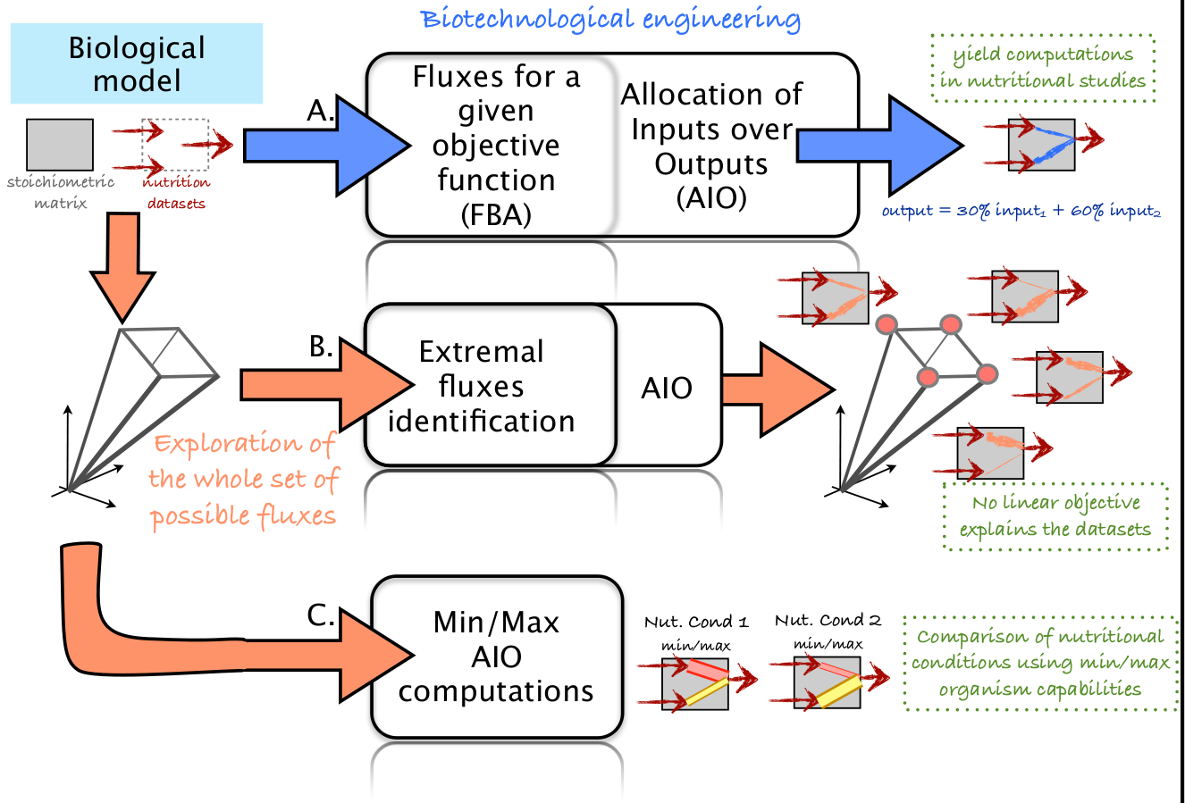 The aim of this tutorial is to explain material and method used to produce all results in the submitted article: ”Exploring metabolism flexibility in complex organisms through quantitative study of precursor sets for system outputs”.
It consists of three parts. In Part I we present the procedure to compute the allocation of Inputs over Output (AIO) for an extremal flux distribution, distribution which maximizing a linear objective function in a simplex (It corresponds to a vertex of the simplex). In Part II we present the procedure for determining all vertices of the simplex so as to determine their AIO and the last part presents the procedure for determining the interval ranges of AIO through the whole simplex. All these three part are illustrated with an example based on a theoretical mammary epithelial cell of a monogastric mammal. The cell taken up AA for protein (peptide) synthesis (9 mmol/h), an excess of leucine (Leucine input = 1 mmol/h) and glucose (input: 80 mmol/h). This cell produced out of the system protein (peptide output = 10 mmol/h), lactose (Lactose ouput= 10 mmol/h), triglycerides (lipid output: 3 mmol/h) composed of 3 C(16:0)-acyl CoA ( C(16:0) output = 9 mmmol/h). In addition, there was a requirement to synthesize serine (Serine output: 1 mmol/h), to do peptide synthesis (since peptide output = 10 mmol/h) and Leucine input was in excess ( and should be catabolized).
A web application dedicated to the computation of allocation for an extremal flux distribution is available at: http://nutritionanalyzer.genouest.org
Here are the main functionnalities of this web application.
In this page, the user has the choice to use a predefined model (simple input mode) are to use its own model either in the propriatary .mdl file format or by providing the stoichiometric matrix of the system in a .csv format (the field separator must be a comma). Notice that these latter files can easily be obtained by using some standard tools (eg. COBRA toolbox). Examples of .mdl and .csv file are provided here: ExampleTutorial_mdlANDcsv_files.zip

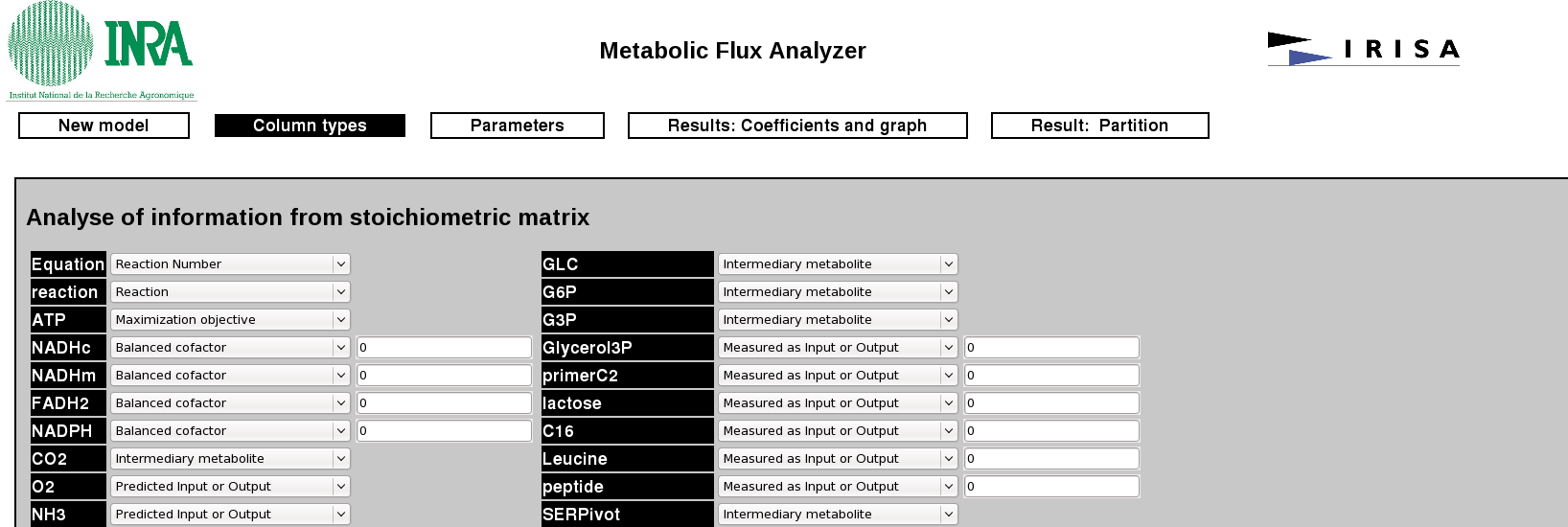
In this page, the user has to define the type of each metabolites (input/output, co-factor, pivots,...) of the system. More precisely, the type of each columns of the stoichiometric matrix can be defined here.
Here the user can define some constraints on the reactions fluxes both in a graphical way (by disabling a reaction or imposing a flux value) or by providing a numerical constraint. Examples:
R_19 + 2 * R_20 = R_30CO2 < 1500Maximize ATP + R_20
Extremal flux distribution corresponds to the vector formed by the values of the flux of each reaction. These values provide the optimal value of the linear objective function.

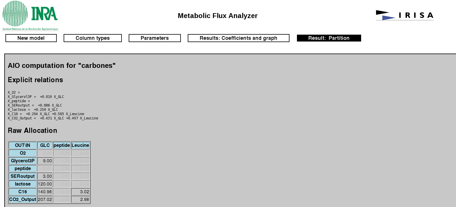
It displays four types of relationship, an explicit form of linear equation for calculating allocations; a table, whose columns correspond to the inputs and rows to the outputs, giving the amount of allocation of inputs over each output; a table giving the percentage of allocation of inputs over outputs and a table giving the percentages outputs allocation from inputs
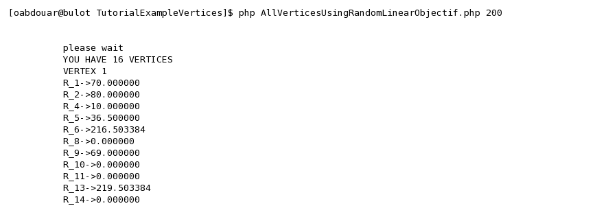
To compute all vertices, we generated some random linear objective function to be optimize, on the simplex by using the simplex algorithm. For the model ExampleTutorial.mdl above all vertices can be generated by downloading the .zip below. Notice that to execute the files PHP CLI( Hypertext Preprocesso Command Line Interface) must be properly installed.
The zip is provided here: TutorialExampleVertices.zip
It contains three files
numberOfRandomObjectiveFunction is an integer number (it can be 5, 19, 30, 200, 500, ... example of running: php AllVerticesUsingRandomLinearObjectif.php 200)
In addition to this tutorial, Sommets.zip implements a complete parallel method (for both a multicore computer or a cluster of several computers) for computing all the vertices where a well formed .mdl is given. The interest reader should refer to the included README.txt file for details.
The intervals give the min-max range of AIO through all the simplex. The min-max are obtain by optimizing some no convex functions. An additional problem is to obtain analytical formula for functions to be optimized. Analytical formula are obtain by computing the inverse of a matrix which is always intertible, called M-matrix, using sagemath. We have developed a local search algorithm, which showed that the points corresponding to these minima and maxima are on the edge of the simplex, contrary to libraries that find points near the edge of the simplex. For the model ExampleTutorial.mdl intervals of AIO can be computed by downloading the .zip below. Notice that to execute files matlab and sagemath must be properly installed.
The zip is provided here: IntervalsAIO_ExampleTutorial.zip
It contains three files
Before starting to run the scripts, it is important to have the three files in the same directory.
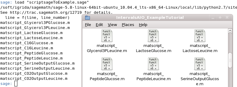
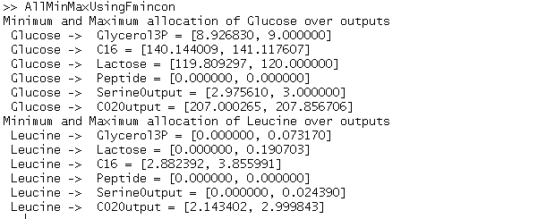
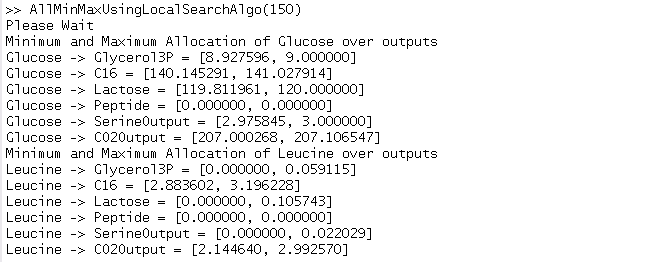
arg is an input integer parameter for the script. More his value is large more the results obtain close with fmincon results
This web page contains links to the .mdl files used in our study on dairy cows.
The three nutritional conditions are synthesized in the following table (Table 2).
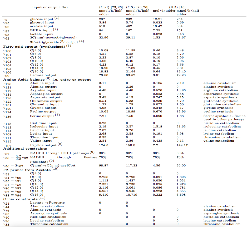
Here, each file corresponds to a distinct vertex of the flux cone. These files corresponds to results synthesized in the following table (Table 4).
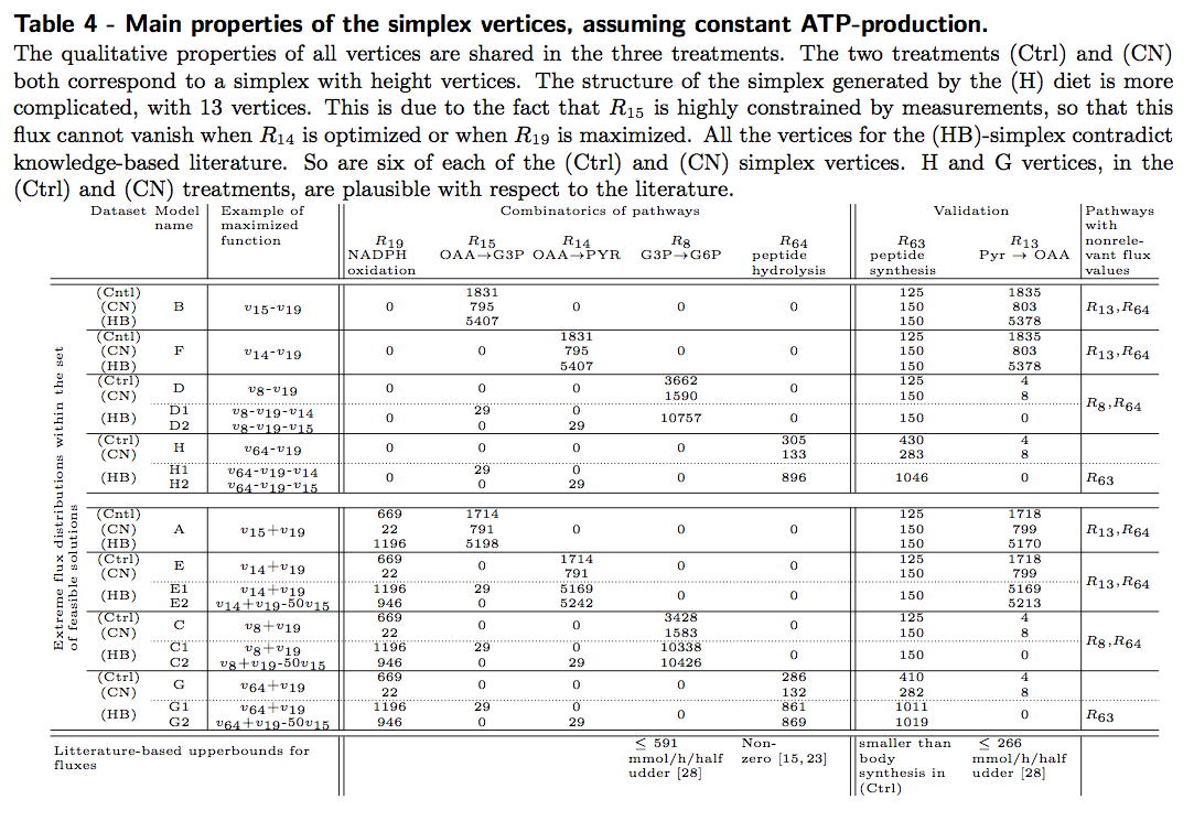
The .mdl files corresponding to the 8 extremal vertices in the CTRL condition: CTRL_condition_allvertices.zip
The .mdl files corresponding to the 8 extremal vertices in the CN condition: CN_condition_allvertices.zip
The .mdl files corresponding to the 13 extremal vertices in the HB condition: HB_condition_allvertices.zip
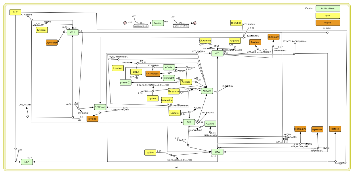
Figure 2 is rendered by CellDesigner v4.2 by using a sbml description of the metabolic network. The sbml file is available here: MammaryGlandModel.sbml.
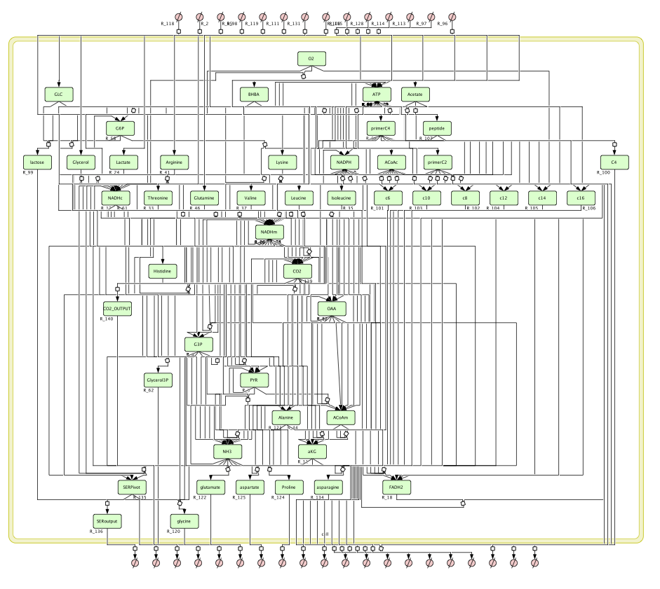
The model can be slightly modified in order to integrate Long Chain Fatty Acids retro control. This gives rise to three new models depending on the quantity of recycled Fatty Acids.